Big O notation is an asymptotic notation used to describe the performance or complexity of an algorithm. Big O specifically describes the worst-case scenario, and can be used to describe the execution time required or the space used by an algorithm. Big-O analysis should be straightforward as long as we correctly identify the operations that are dependent on n, the input size.
The general step wise procedure for Big-O runtime analysis is as follows:
- Figure out what the input is and what n represents.
- Express the maximum number of operations, the algorithm performs in terms of n.
- Eliminate all excluding the highest order terms.
- Remove all the constant factors.
Runtime Analysis of Algorithms (Time Complexity)
The fastest possible running time for any algorithm is O(1), commonly referred to as Constant Running Time. In this case, the algorithm always takes the same amount of time to execute, regardless of the input size. This is the ideal runtime for an algorithm, but it’s rarely achievable.
In actual cases, the performance (Runtime) of an algorithm depends on n, that is the size of the input or the number of operations is required for each input item.
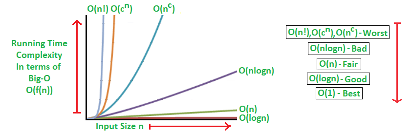
The algorithms can be classified as follows from the best-to-worst performance (Running Time Complexity):
- Constant- no loops- O(1)
- A logarithmic algorithm – O(logn)
Runtime grows logarithmically in proportion to n. Usually searching algorithms have log n if they are sorted (Binary Search). - A linear algorithm – O(n)
Runtime grows directly in proportion to n. for loops, while loops through n items - A superlinear algorithm – O(nlogn)
Runtime grows in proportion to n. Usually sorting operations - A polynomial algorithm – O(n^c)
Runtime grows quicker than previous all based on n. Every element in a collection needs to be compared to ever other element. Two nested loops - A exponential algorithm – O(c^n)
Runtime grows even faster than polynomial algorithm based on n. Every element in a collection needs to be compared to ever other element. Two nested loops. - A factorial algorithm – O(n!)
Runtime grows the fastest and becomes quickly unusable for even
small values of n. You are adding a loop for every element.
*note- Where, n is the input size and c is a positive constant.
What can cause time in a function?
Operations (+, -, *, /)
Comparisons (<, >, ==)
Looping (for, while)
Outside Function call (function())
Rule Book
Rule 1: Always worst Case
Rule 2: Remove Constants
Rule 3: Different inputs should have different variables. O(a+b). A and B
arrays nested would be
O(a*b)
+ for steps in order
* for nested steps
Rule 4: Drop Non-dominant terms
Algorithmic Examples of Runtime Analysis:
Some of the examples of all those types of algorithms (in worst-case scenarios) are mentioned below:
- Logarithmic algorithm – O(logn) – Binary Search.
- Linear algorithm – O(n) – Linear Search.
- Superlinear algorithm – O(nlogn) – Heap Sort, Merge Sort.
- Polynomial algorithm – O(n^c) – Strassen’s Matrix Multiplication, Bubble Sort, Selection Sort, Insertion Sort, Bucket Sort.
- Exponential algorithm – O(c^n) – Tower of Hanoi.
- Factorial algorithm – O(n!)
O(1) time– Constant Running Time
O(1) describes an algorithm that will always execute in the same time (or space) regardless of the size of the input data set.
bool IsFirstElementNull(IList<string> elements)
{
return elements[0] == null;
}
- Accessing Array Index (int a = ARR[5];)
- Inserting a node in Linked List
- Pushing and Poping on Stack
- Insertion and Removal from Queue
- Finding out the parent or left/right child of a node in a tree stored in Array
- Jumping to Next/Previous element in Doubly Linked List
O(n) time– Linear algorithm
In a nutshell, all Brute Force Algorithms, or Noob ones which require linearity, are based on O(n) time complexity
- Traversing an array
Traversing a linked list - Linear Search
- Deletion of a specific element in a Linked List (Not sorted)
- Comparing two strings
- Checking for Palindrome
- Counting/Bucket Sort and here too you can find a million more such examples….
O(log n) time– Logarithmic algorithm
- Binary Search
- Finding largest/smallest number in a binary search tree
- Certain Divide and Conquer Algorithms based on Linear functionality
- Calculating Fibonacci Numbers – Best Method The basic premise here is NOT using the complete data, and reducing the problem size with every iteration
O(n log n) time– Superlinear algorithm
The factor of ‘log n’ is introduced by bringing into consideration Divide and Conquer. Some of these algorithms are the best optimized ones and used frequently.
- Merge Sort
- Heap Sort
- Quick Sort
- Certain Divide and Conquer Algorithms based on optimizing O(n^2) algorithms
O(n^2) time– Polynomial algorithm
These ones are supposed to be the less efficient algorithms if their O(nlogn) counterparts are present. The general application may be Brute Force here.
- Bubble Sort
- Insertion Sort
- Selection Sort
- Traversing a simple 2D array
O(n!) time- Permutation algorithm
O(n!)denotes an algorithm that iterates over all possible combinations of the inputs.
O(2^N) time- Exponential algorithm
O(2^N) denotes an algorithm whose growth doubles with each addition to the input data set. The growth curve of an O(2^N) function is exponential – starting off very shallow, then rising meteorically. An example of an O(2^N) function is the recursive calculation of Fibonacci numbers:
Memory Footprint Analysis of Algorithms (Space complexity)
For performance analysis of an algorithm, we need to consider both time complexity and space complexity. Here also, we need to measure and compare the worst case theoretical space complexities of algorithms for the performance analysis.
It basically depends on two major aspects described below:
- Firstly, the implementation of the program is responsible for memory usage. For example, we can assume that recursive implementation always reserves more memory than the corresponding iterative implementation of a particular problem.
- And the other one is n, the input size or the amount of storage required for each item. For example, a simple algorithm with a high amount of input size can consume more memory than a complex algorithm with less amount of input size.
Examples of Space complexity (worst-case scenarios):
- Ideal algorithm – O(1) – Linear Search, Binary Search, Bubble Sort, Selection Sort, Insertion Sort, Heap Sort, Shell Sort.
- Logarithmic algorithm – O (log n) – Merge Sort.
- Linear algorithm – O(n) – Quick Sort.
- Sub-linear algorithm – O(n+k) – Radix Sort.
Time complexity vs Space complexity:
the more time efficiency you have, the less space efficiency you have and vice versa.
For example, Merge-sort algorithm is exceedingly fast but requires a lot of space to do the operations. On the other side, Bubble Sort is exceedingly slow but requires the minimum space.
What causes Space complexity?
1.Variables
2. Data Structures
3. Function Call
4. Allocations
Big O Reference of common algorithms and data structures
Sorting
Very important and useful type of algorithms for many common problems nowadays, Finder, iTunes, Excel and many more programs use some kind of sorting algorithm.
| Algorithm | Time | Auxiliary Space | ||
|---|---|---|---|---|
| Best | Average | Worst | Worst | |
| Bubble sort | O(n) | O(n2) | O(n2) | O(1) |
| Insertion sort | O(n) | O(n2) | O(n2) | O(1) |
| Selection sort | O(n2) | O(n2) | O(n2) | O(1) |
| Mergesort | O(n log(n)) | O(n log(n)) | O(n log(n)) | O(n) |
| Quicksort | O(n log(n)) | O(n log(n)) | O(n2) | O(log(n)) |
| Heapsort | O(n log(n)) | O(n log(n)) | O(n log(n)) | O(1) |
Shell Sort(h=2^k-1) | O(n log(n)) | O(n1.25) conjectured | O(n(3/2)) | O(1) |
| Bucket sort | O(n+k) | O(n+k) | O(n2) | O(nk) |
| Radix sort | O(nk) | O(nk) | O(nk) | O(n+k) |
Searching
Searching efficiently is crucial for many operations in different parts of the software we use on a daily basis.
| Algorithm | Data Structure | Time | Space | |
|---|---|---|---|---|
| Average | Worst | Worst | ||
| Depth First Search (DFS) | Graph of |V| vertices and |E| edges | - | O(|E| + |V|) | O(|V|) |
| Breadth First Search (BFS) | Graph of |V| vertices and |E| edges | - | O(|E| + |V|) | O(|V|) |
| Binary Search | Sorted array of n elements | O(log(n)) | O(log(n)) | O(1) |
| Linear (Brute force) | Array of n elements | O(n) | O(n) | O(1) |
| Shortest path by Dijkstra, Min-heap as priority queue | Graph of |V| vertices and |E| edges | O((|V|+|E|) log|V|) | O((|V|+|E|) log|V|) | O(|V|) |
| Shortest path by Dijkstra, unsorted array as priority queue | Graph of |V| vertices and |E| edges | O(|V|2) | O(|V|2) | O(|V|) |
| Shortest path by Bellman-Ford | Graph of |V| vertices and |E| edges | O(|V||E|) | O(|V||E|) | O(|V|) |
Common Data Structures
Data structures are the key in some of the most used algorithms and a good data structure is sometimes the way to achieve a very efficient and elegant solution.
| Data Structure | Time | |||||||
|---|---|---|---|---|---|---|---|---|
| Average | Worst | |||||||
| Indexing | Search | Insertion | Deletion | Indexing | Search | Insertion | Deletion | |
| Basic Array | O(1) | O(n) | - | - | O(1) | O(n) | - | - |
| Dynamic Array | O(1) | O(n) | O(n) | O(n) | O(1) | O(n) | O(n) | O(n) |
| Single-Linked List | O(n) | O(n) | O(1) | O(1) | O(n) | O(n) | O(1) | O(1) |
| Double-Linked List | O(n) | O(n) | O(1) | O(1) | O(n) | O(n) | O(1) | O(1) |
| Skip List* | O(log(n)) | O(log(n)) | O(log(n)) | O(log(n)) | O(n) | O(n) | O(n) | O(n) |
| Hash Table | - | O(1) | O(1) | O(1) | - | O(n) | O(n) | O(n) |
| Binary Search Tree | O(log(n)) | O(log(n)) | O(log(n)) | O(log(n)) | O(n) | O(n) | O(n) | O(n) |
| Ternary Search Tree | - | O(log(n)) | O(log(n)) | O(log(n)) | - | O(n) | O(n) | O(n) |
| Cartesian Tree | - | O(log(n)) | O(log(n)) | O(log(n)) | - | O(n) | O(n) | O(n) |
| B-Tree | O(log(n)) | O(log(n)) | O(log(n)) | O(log(n)) | O(log(n)) | O(log(n)) | O(log(n)) | O(log(n)) |
| Red-Black Tree | O(log(n)) | O(log(n)) | O(log(n)) | O(log(n)) | O(log(n)) | O(log(n)) | O(log(n)) | O(log(n)) |
| Splay Tree | - | O(log(n)) | O(log(n)) | O(log(n)) | - | O(log(n)) | O(log(n)) | O(log(n)) |
| AVL Tree | O(log(n)) | O(log(n)) | O(log(n)) | O(log(n)) | O(log(n)) | O(log(n)) | O(log(n)) | O(log(n)) |
Note * All have space complexity of O(n) except for Skip that has O(n log(n))
Heaps
| Heaps | Time | ||||||
|---|---|---|---|---|---|---|---|
| Heapify | Find Max | Extract Max | Increase Key | Insert | Delete | Merge | |
| Linked List | - | O(1) | O(1) | O(n) | O(n) | O(1) | O(m+n) |
| Linked List (unsorted) | - | O(n) | O(n) | O(1) | O(1) | O(1) | O(1) |
| Binary Heap | O(n) | O(1) | O(n log(n)) | O(n log(n)) | O(n log(n)) | O(n log(n)) | O(m+n) |
| Binomial Heap | - | O(n log(n)) | O(n log(n)) | O(n log(n)) | O(n log(n)) | O(n log(n)) | O(n log(n)) |
| Fibonnaci Heap | - | O(1) | O(log(n))* | O(1)* | O(1) | O(log(n))* | O(1) |
Note * Amortized time
Graphs
| Node / Edge Management | Storage | Add Vertex | Add Edge | Remove Vertex | Remove Edge | Query |
|---|---|---|---|---|---|---|
| Adjacency List | O(|V|+|E|) | O(1) | O(1) | O(|V|+|E|) | O(|E|) | O(|V|) |
| Incidence List | O(|V|+|E|) | O(1) | O(1) | O(|E|) | O(|E|) | O(|E|) |
| Adjacency Matrix | O(|V|2) | O(|V|2) | O(1) | O(|V|2) | O(1) | O(1) |
| Incidence Matrix | O(|V|⋅|E|) | O(|V|⋅|E|) | O(|V|⋅|E|) | O(|V|⋅|E|) | O(|V|⋅|E|) | O(|E|) |
